Explainability in Neural Networks, Part 2: Limitations of Simple Feature Attribution Methods
We examine some simple, intuitive methods to explain the output of a neural network (based on perturbations and gradients), and see how they produce non-sensical results for non-linear functions.


$
\def\R{{\mathbb{R}}}
$
Recap of perturbation-based attribution
In the previous post we kicked off our discussion of explainability in DNNs by presenting a simple feature attribution method for evaluating the contribution of an input feature to a neural network's output. Specifically, we considered an intuitive method for feature attribution (some authors refer to it as a perturbation[1] or ablation[2] method): If $ F(x)$ is the (scalar) function computed by the neural network (where $x \in \R^d$ is a $d$-dimensional input feature vector), we posit a certain "information-less" or "neutral" baseline input vector $b \in \R^d$, and measure the attribution of $F(x)$ to feature $x_i$ (relative to the baseline $b$) denoted $A^F_i(x; b)$, as the difference between $F(x)$ and the counterfactual output $F(x[x_i = b_i])$obtained by perturbing $x_i$ to its baseline value $b_i$:
$$
A^F_i(x; b) := F(x) - F(x[x_i = b_i])
$$
We saw that when this method is applied to a simple linear model, it satisfies a nice property called additivity: the feature attributions add up to $F(x) - F(b)$, the change in the DNN output from input $b$ to input $x$. And this property (also referred to as completeness by some authors[3] ) is nice to have since we can think of each feature's attribution as its contribution to the output change $F(x) - F(b)$. We concluded by saying that this property would not hold in general when there are non-linearities, which of course are essential to the operation of a DNN.
Saliency methods in general
At this point it will be helpful to pause and see where this method fits within the broader class of feature-importance measures (we borrow some of this description from recent papers[1:1][4] [5]). Attribution methods belong to a more general class of explanation methods known as saliency methods: roughly speaking, these methods seek to provide insights into the output $F(x)$ by ranking the explanatory power (or "salience" on "importance") of input features. Some of the saliency methods proposed recently include:
- Gradients or sensitivity: A feature's importance is measured by computing the sensitivity of the output score to a change in the input feature value. For example one could look at the gradient $\partial F(x)/\partial(x_i)$ as a measure of how relevant a feature $x_i$ is to the output $F(x)$. We look at this method in more detail below.
- Signal Methods: These methods have mainly been applied in visual domains to better understand the representations learned by internal layers in a Convolutional Neural Network (CNN, or "convnet"), by identifying patterns in the input pixel space that cause specific internal neuron activations. For example Zeiler et al., 2013[6] do this by mapping internal neuron activations back to the input pixel space.
- Attribution Methods: These methods explicitly try to estimate the contribution of each input feature to the network's output (or possibly the change in output from a baseline output). The perturbation method above is one such method.
Note that when applying these methods, $F(x)$ could either represent the final output sore (e.g. probability of a certain class-label), or it could represent the activation value of an internal neuron.
Non-sensical Attributions with the Perturbation Method
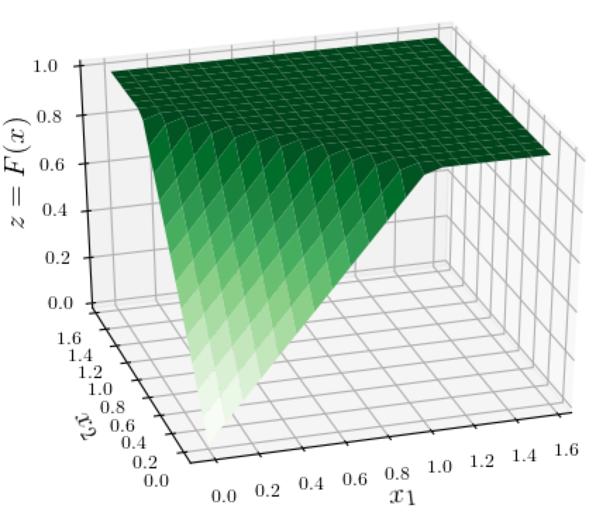
Now let's return to the perturbation-based attribution method above and examine some of its limitations. Consider the following example (related to the one in Shrikumar et al., 2017[1:2]). Say we have a simple non-linear function $F(x)$ of a 2-dimensional input vector $x$ where $x_i \geq 0$ for $i \in \{1,2\}$, and
$$
F(x) = \min(1, x_1 + x_2)
$$
Below is a 3D surface plot of this function. What's significant about this function is that, as the sum of the coordinates $s = x_1 + x_2$ increases from 0, the value of $F(x)$ is initially $s$, but then flattens out after $s=1$. The darker green colors in the plot indicate higher values of $F(x)$.
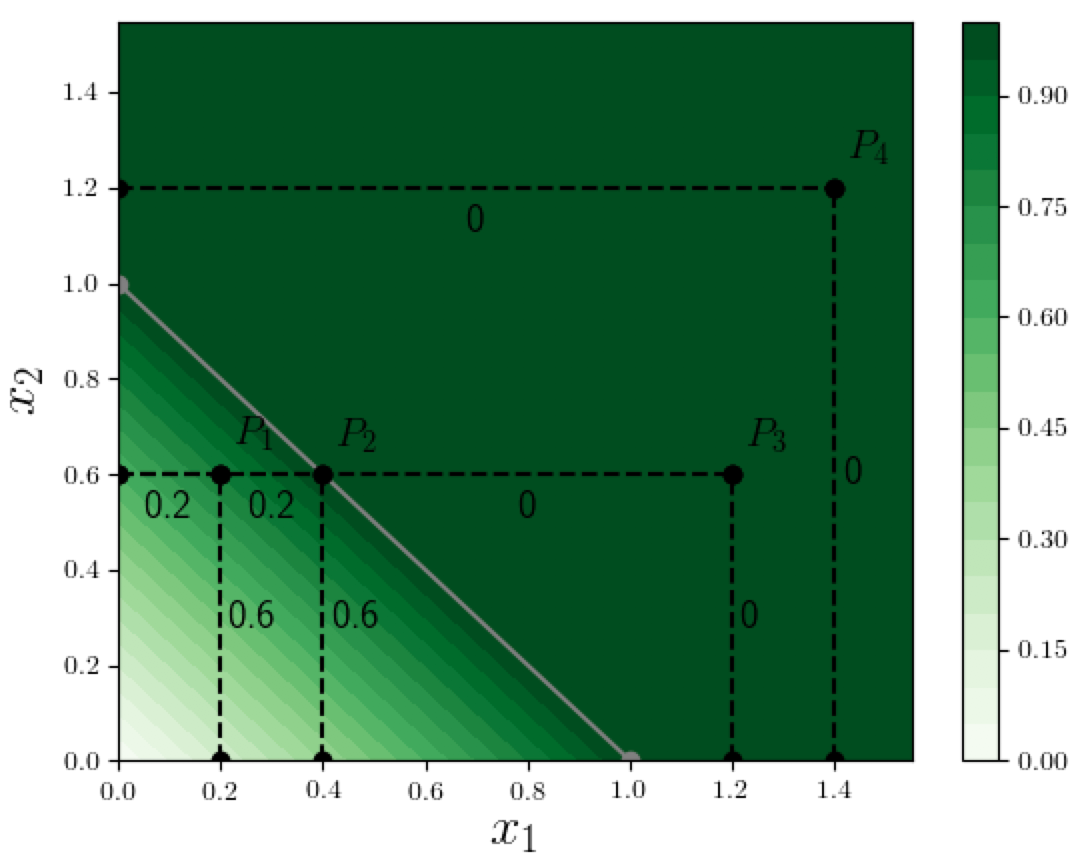
It will be more convenient for us to look at at a 2D contour plot instead, as shown below. This is essentially a view "from the top" of the above 3D surface plot, where the value of the function $F(x)$ is encoded by the darkness of the green color: Darker bands correspond to points $x$ with higher values of $F(x)$. All the points to the right and above the white line have the same dark green color, indicating that the function is 1 in that entire region. The spacing between bands in the countour plot is also meaningful: the function-value changes by the same amount between bands, so a bigger spacing means that the function is changing more slowly. (Of course in the non-flat region, the function is linear so the spacing is uniform there, but in the logistic function example below, we will see non-uniform spacing.)
Now here is a geometric view of the perturbation-based attribution method:
The attribution $A^F_i(x; b)$ to a feature $x_i$ is the drop in the value of the function $F(.)$ when we move on a straight line path (parallel to the $x_i$-axis) from $x$ to $x[x_i=b_i]$.
In our specific 2D example above, assuming a baseline vector $b=(0,0)$ (where $F(b)=0$), this translates to:
For any point $P$ with coordinates $(x_1, x_2)$, the attribution to dimension $i$ ($i \in \{1,2\}$) is the drop in the value of the function $F(x)$ when we move on a straight line path from $P$ parallel to the $x_i$ axis until $x_i=0$, i.e., to find the attribution to dimension $i$ we move from $P$ along the perpendicular to the other dimension.
To make it easier to read off the attributions, we show the amount by which the function value drops along each dotted line-segment (assuming we are moving toward one of the axes). For example at point $P_1 = (0.2, 0.6)$ the attributions to dimensions 1 and 2 are 0.2 and 0.6 respectively, which is what we would expect. Similarly at $P_2 = (0.4, 0.6)$ the attributions are 0.4 and 0.6.
But the point $P_3 = (1.2, 0.6)$ is interesting: the change in function value is 0 as we move from $P_3$ to $ P_2$ and the total change on the perpendicular path to the $x_2$ axis is 0.4, so the attribution to $x_1$ is 0.4. However the attribution to $x_2$ is zero since the function value doesn't change at all along the perpendicular path from $P_3$ to the $x_1$-axis! Point $P_4 = (1.4, 1.2)$ is an even more extreme example: the attributions to both dimensions are zero. The reason for these oddities is clearly the flattening out of the function $F(x)$ when the sum of its input dimensions exceeds 1. This is an instance of the well-known saturation issue in the attribution methods literature:
Saturation: When the output of a neural network is (completely or nearly) saturated, some attribution methods may significantly underestimate the importance of features.
In our example, when using the perturbation method, the contributions of the coordinates "saturate" when their sum reaches 1, and so for any point $x$ where either coordinate is at least 1 (such as $P_3$ or $P_4$ above), the contribution of the other coordinate will be 0 (since its perturbation to 0 will not affect the function value).
Besides the zero attribution problem, points $P_3$ and $P_4$ raise a subtler issue: how do we allocate "credit" for the function value (which is 1 at both points) among the two coordinates? For example for $P_3 = (1.2, 0.6)$, we know that the perturbation-based allocation of $(0.4, 0)$ is somehow "wrong" (besides violating additivity, it is counterintuitive that the second dimension gets no credit), but then what is the "correct" or fair allocation of credit? The $x_1$ coordinate is twice the $x_2$ coordinate, so does that mean we should allocate twice the credit to the first coordinate?
Gradient/Sensitivity based Saliency Method
Before considering these questions, let us look at a different saliency method, mentioned above:
Gradient or Sensitivity based importance: The importance of a feature $x_i$ to the output $F(x)$ of a DNN, relative to a baseline vector $b$, is defined as:
\begin{equation*} G^F_i(x; b) := (x_i - b_i) \partial F(x)/\partial x_i \end{equation*}
This is not that different in spirit from the perturbation method: instead of perturbing the input feature $x_i$ to its baseline value $b_i$ and looking at how the output $F(x)$ changes, here we are computing the gradient $g$ of $F(x)$ with respect to $x_i$ and estimating the function value change, by an approximation $ g(x_i - b_i)$which would be exact if the gradient was constant between the current feature value $x_i$ and the baseline feature value $b_i$. Of course, if the gradient really were constant then there would be no difference between the perturbation method and the gradient method. (This method can also be rationalized by a first-order Taylor expansion of the multi-variate function $F(x)$).
The gradient method is not immune to the saturation issue either, since for any point $(x_1, x_2)$ in the saturated region (i.e. where $x_1 + x_2 > 1$) the gradients w.r.t. both $x_1$ and $x_2$ would both be zero, and hence the method would assign zero importance to both features.
Other Non-Linearities: Logistic Function
We should note that the above oddities in attribution are exhibited not just by a function $F(x)$ that "flattens out" suddenly; any non-linearity can cause similar issues. For example the logistic function
$$
F(x) = \frac{1}{1 + \exp(-x_1 - x_2 - 1)},
$$
displayed in this 3D surface plot below, causes similar difficulties for the perturbation and gradient-based methods.
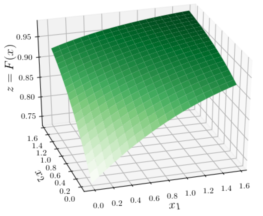
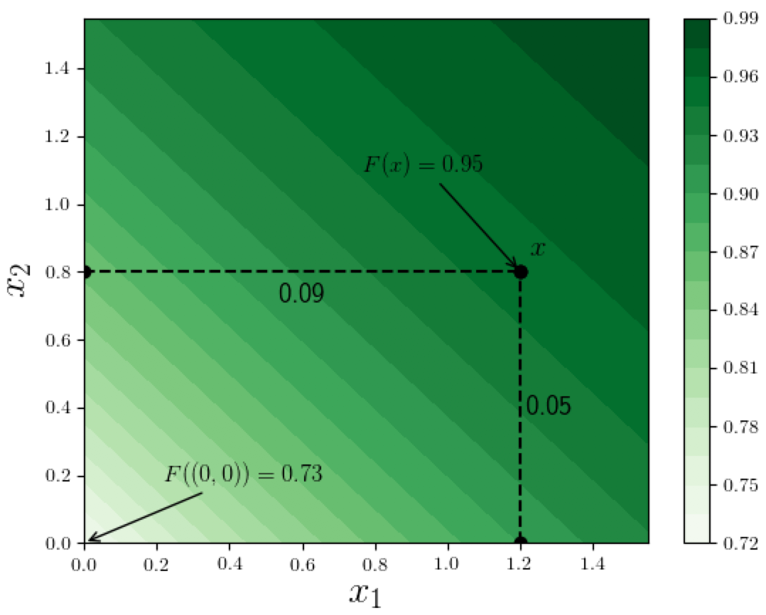
In the corresponding 2D contour plot (see below), the "gradual" flattening out is shown by the increasingly-spaced bands toward the upper-right side of the figure. Notice how for the point $x=(1.2, 0.8)$, the difference $F(x) - F((0,0)) = 0.22$, but the attributions to the 2 coordinates sum to just 0.14, violating the additivity/completeness property.
Exploring alternative methods
At this point it may seem like a challenging task to define a feature attribution method that satisfies additivity and perhaps other desirable properties. Let us revisit the geometric view of the perturbation-method above, to see if it might offer a possible clue for a better attribution method. We said that when attributing the $F(x) - F(b)$ to a dimension $x_i$ we move from the point $x$ along a straight line path parallel to the $x_i$ axis until the $i$'th coordinate equals $b_i$. In other words we are trying to allocate "credit" for $F(x)-F(b)$ according to the function-value change along $i$ different straight line paths.
For example for point $P_3 = (1.2, 0.6)$ in the saturation example above, the attributions were based on the function-change along a "horizontal" path and a "vertical" path to the axes. Can we try to define a single path and allocate credit according to how the function changes on that path? Let us try a couple of possible paths from point $P_3$ to the origin, as shown in the figure below:
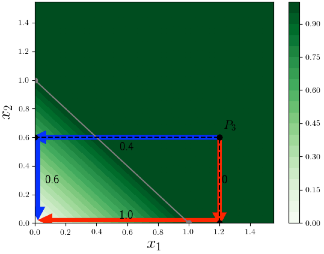
- Suppose we pick the red path from $P_3$ that first goes "down" to the $x_1$ axis, then to the "left" to meet the origin. We could say, "when we go down, only $x_2$ is changing and the function value remains at 1, so $x_2$ should get no credit, but when we go left to the origin, only $x_1$ is changing, and the function value drops to 0, so $x_1$ should get credit 1." This doesn't seem right!
- Now try the blue path from $P_3$ that goes "left" to the $x_2$ axis first, then goes "down" to the origin. This gives attributions (0.4, 0.6). Now this does satisfy additivity, but it does not seem fair since $x_1=1.2$ is twice as large as $x_2 = 0.6$, so we think $x_1$ should get at least a larger credit, or maybe even a proportionally larger credit. To make this argument more persuasive, try a point $x = (100,0.6)$, for which this left-then-down path method gives the same $(0.4, 0.6)$ attributions.
So just picking an arbitrary path is not going to give us a sensible attribution. But it turns out that paths, and gradients along paths, are central to one way of defining attributions that satisfy additivity and other desirable properties. We will look at this in a future post.
Shrikumar, Avanti, Peyton Greenside, and Anshul Kundaje. 2017. “Learning Important Features Through Propagating Activation Differences.” arXiv [cs.CV]. arXiv. http://arxiv.org/abs/1704.02685. ↩︎ ↩︎ ↩︎
Sundararajan, Mukund, Ankur Taly, and Qiqi Yan. 2016. “Gradients of Counterfactuals.” arXiv [cs.LG]. arXiv. http://arxiv.org/abs/1611.02639. ↩︎
Sundararajan, Mukund, Ankur Taly, and Qiqi Yan. 2017. “Axiomatic Attribution for Deep Networks.” arXiv [cs.LG]. arXiv. http://arxiv.org/abs/1703.01365. ↩︎
Kindermans, Pieter-Jan, Kristof T. Schütt, Maximilian Alber, Klaus-Robert Müller, Dumitru Erhan, Been Kim, and Sven Dähne. 2017. “Learning How to Explain Neural Networks: PatternNet and PatternAttribution.” arXiv [stat.ML]. arXiv. http://arxiv.org/abs/1705.05598. ↩︎
Kindermans, Pieter-Jan, Sara Hooker, Julius Adebayo, Maximilian Alber, Kristof T. Schütt, Sven Dähne, Dumitru Erhan, and Been Kim. 2017. “The (Un)reliability of Saliency Methods.” arXiv [stat.ML]. arXiv. http://arxiv.org/abs/1711.00867. ↩︎
Zeiler, Matthew D., and Rob Fergus. 2013. “Visualizing and Understanding Convolutional Networks.” arXiv [cs.CV]. arXiv. http://arxiv.org/abs/1311.2901. ↩︎